90. The Aiyagari Model with Endogenous Grid Method#
In addition to what’s included in base Anaconda, we need to install QuantEcon’s Python library and JAX.
!pip install quantecon jax
90.1. Overview#
This lecture combines two important computational methods in macroeconomics:
The Aiyagari model [Aiyagari, 1994] – a heterogeneous agent model with incomplete markets
The endogenous grid method (EGM) [Carroll, 2006] – an efficient algorithm for solving dynamic programming problems
In the standard Aiyagari lecture, we solved the household problem using discretization and value function iteration.
We then computed aggregate capital at a given set of prices using the stationary distribution of the finite Markov chain.
In this lecture, we take a different approach:
We use the endogenous grid method to solve the household problem via the Euler equation and linear interpolation.
We compute aggregate capital by simulation rather than an algebraic technique (which only works for the finite case).
These modifications make the solution method faster and more flexible, especially when dealing with more complex models.
We use JAX throughout, so that the EGM operator, the solver and the simulation are all JIT-compiled and vectorized.
90.1.1. References#
The primary references for this lecture are:
our previous Aiyagari lecture for the key ideas
[Aiyagari, 1994] for the economic model
[Carroll, 2006] for the endogenous grid method
Chapter 18 of [Ljungqvist and Sargent, 2018] for textbook treatment
90.1.2. Preliminaries#
We use the following imports:
import quantecon as qe
import matplotlib.pyplot as plt
import jax
import jax.numpy as jnp
import numpy as np
from typing import NamedTuple
from functools import partial
from scipy.optimize import bisect
We will use 64-bit floats with JAX in order to increase precision.
jax.config.update("jax_enable_x64", True)
90.2. The Economy#
The economy consists of households and a representative firm.
90.2.1. Households#
Infinitely lived households face idiosyncratic income shocks and a borrowing constraint.
The savings problem faced by a typical household is
subject to
where
\(c_t\) is current consumption
\(a_t\) is assets
\(z_t\) is an exogenous component of labor income (stochastic employment status)
\(w\) is the wage rate
\(r\) is the interest rate
\(B\) is the maximum amount that the agent is allowed to borrow
The exogenous process \(\{z_t\}\) follows a finite state Markov chain with stochastic matrix \(\Pi\).
Optimal interior consumption choices satisfy the Euler equation
(We use \('\) symbols for both derivatives and future values, which is not ideal but convenient and common.)
In terms of assets, this is
where \(s\) is the optimal savings policy function.
90.2.2. Firms#
Firms produce output by hiring capital and labor under constant returns to scale.
The representative firm’s output is
where
\(A\) and \(\alpha\) are parameters with \(A > 0\) and \(\alpha \in (0, 1)\)
\(K\) is aggregate capital
\(N\) is total labor supply (normalized to 1)
These parameters are stored in the following namedtuple:
class Firm(NamedTuple):
    A: float = 1.0    # Total factor productivity
    N: float = 1.0    # Total labor supply
    α: float = 0.33   # Capital share
    δ: float = 0.05   # Depreciation rate
From the firm’s first-order condition, the inverse demand for capital is
def r_given_k(K, firm):
    """
    Inverse demand curve for capital.
    """
    A, N, α, δ = firm
    return A * α * (N / K)**(1 - α) - δ
The equilibrium wage rate as a function of \(r\) is
def r_to_w(r, firm):
    """
    Equilibrium wages associated with a given interest rate r.
    """
    A, N, α, δ = firm
    return A * (1 - α) * (A * α / (r + δ))**(α / (1 - α))
90.2.3. Equilibrium#
A stationary rational expectations equilibrium (SREE) consists of prices and policies such that:
Households optimize given prices
Firms maximize profits given prices
Markets clear: aggregate capital supply equals aggregate capital demand
Aggregate quantities are constant over time
90.3. Implementation with EGM#
90.3.1. Household primitives#
First we set up the household parameters and grids:
class Household(NamedTuple):
    β: float            # Discount factor
    a_grid: jnp.ndarray # Asset grid
    z_grid: jnp.ndarray # Exogenous states
    Π: jnp.ndarray      # Transition matrix

def create_household(β=0.96,                      # Discount factor
                     Π=[[0.9, 0.1], [0.1, 0.9]],  # Markov chain
                     z_grid=[0.1, 1.0],           # Exogenous states
                     a_min=1e-10, a_max=50.0,     # Asset grid
                     a_size=200):
    """
    Create a Household namedtuple with custom grids.
    """
    a_grid = jnp.linspace(a_min, a_max, a_size)
    z_grid, Π = map(jnp.array, (z_grid, Π))
    return Household(β=β, a_grid=a_grid, z_grid=z_grid, Π=Π)
For utility, we assume \(u(c) = \log(c)\), which gives us \(u'(c) = 1/c\) and \((u')^{-1}(x) = 1/x\).
@jax.jit
def u_prime(c):
    return 1 / c

@jax.jit
def u_prime_inv(x):
    return 1 / x
Here’s a namedtuple for prices:
class Prices(NamedTuple):
    r: float = 0.01  # Interest rate
    w: float = 1.0   # Wages
90.3.2. The EGM operator#
The key insight of EGM is to avoid root-finding by choosing the asset grid exogenously and computing the consumption values directly from the Euler equation.
The Coleman-Reffett operator using EGM works as follows:
Start with a consumption policy \(\sigma\) represented on an exogenous grid of (next-period) assets \(\{a_i\}\).
For each asset level \(a_i\) and current employment state \(z_j\):
Compute the right-hand side of the Euler equation: $\(\text{RHS} = \beta (1 + r) \sum_{z'} \Pi(z_j, z') \, u'(\sigma(a_i, z'))\)$
Use the inverse marginal utility to get current consumption: $\(c_{ij} = (u')^{-1}(\text{RHS})\)$
Recover the implied current asset level from the budget constraint: $\(a_{ij} = \frac{c_{ij} + a_i - w z_j}{1 + r}\)$
Reconstruct the new policy \(K\sigma\) on the original asset grid by interpolating \((a_{ij}, c_{ij})\), handling the borrowing constraint where it binds.
The whole operation vectorizes cleanly, so we write it as a single JIT-compiled function and use vmap over the employment states:
@jax.jit
def K_egm(σ, household, prices):
    """
    The Coleman-Reffett operator using EGM for the Aiyagari model.

    Here σ[i, j] is consumption when next-period assets are a_grid[i]
    and the current employment state is z_grid[j].
    """
    β, a_grid, z_grid, Π = household
    r, w = prices
    z_size = len(z_grid)

    # Expectation E[u'(c(a', z')) | z] over the next-period shock
    Eu_prime = (Π @ u_prime(σ).T).T                       # (a_size, z_size)

    # Euler equation -> consumption on the endogenous grid
    c_endo = u_prime_inv(β * (1 + r) * Eu_prime)          # (a_size, z_size)

    # Implied current assets: a = (c + a' - w z) / (1 + r)
    a_endo = (c_endo + a_grid[:, None] - w * z_grid[None, :]) / (1 + r)

    # Interpolate back onto the exogenous grid for each employment state
    def interp_policy(j):
        # Where today's assets fall below the endogenous grid the borrowing
        # constraint binds, so the household saves a_grid[0] and consumes
        # the rest of current income.
        return jnp.where(
            a_grid < a_endo[0, j],
            w * z_grid[j] + (1 + r) * a_grid - a_grid[0],
            jnp.interp(a_grid, a_endo[:, j], c_endo[:, j])
        )

    σ_new = jax.vmap(interp_policy)(jnp.arange(z_size))    # (z_size, a_size)
    return σ_new.T                                        # (a_size, z_size)
90.3.3. Solving the household problem#
We solve for the optimal policy by iterating the EGM operator to convergence.
The solver is fully JIT-compiled and uses jax.lax.while_loop for the iteration:
@jax.jit
def solve_household(household, prices, tol=1e-6, max_iter=10_000):
    """
    Solve the household problem by iterating the EGM operator.

    Returns the optimal consumption policy σ[i, j], where i indexes
    next-period assets and j indexes employment states.
    """
    β, a_grid, z_grid, Π = household
    r, w = prices

    # Initial guess: consume half of current income
    income = w * z_grid[None, :] + (1 + r) * a_grid[:, None]
    σ_init = 0.5 * income

    def condition(state):
        i, σ, error = state
        return (error > tol) & (i < max_iter)

    def body(state):
        i, σ, error = state
        σ_new = K_egm(σ, household, prices)
        error = jnp.max(jnp.abs(σ_new - σ))
        return i + 1, σ_new, error

    i, σ, error = jax.lax.while_loop(condition, body, (0, σ_init, tol + 1))
    return σ
Let’s test this on an example:
household = create_household()
prices = Prices(r=0.01, w=1.0)

with qe.Timer():
    σ_star = solve_household(household, prices)
    jax.block_until_ready(σ_star)
0.3651 seconds elapsed
We can check that the policy is a fixed point of the EGM operator by measuring the residual:
residual = jnp.max(jnp.abs(K_egm(σ_star, household, prices) - σ_star))
print(f"Final Euler residual: {residual:.2e}")
Final Euler residual: 8.34e-07
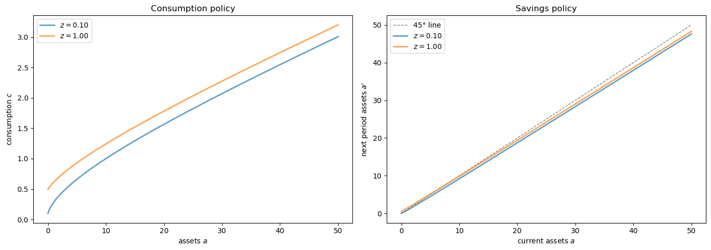
Let’s plot the resulting policy functions:
β, a_grid, z_grid, Π = household
r, w = prices

# Convert consumption policy to savings policy
income = w * z_grid[None, :] + (1 + r) * a_grid[:, None]
savings = income - σ_star

fig, axes = plt.subplots(1, 2, figsize=(14, 5))

# Plot consumption policy
ax = axes[0]
for j, z in enumerate(z_grid):
    ax.plot(a_grid, σ_star[:, j], label=f'$z={z:.2f}$', lw=2, alpha=0.7)
ax.set_xlabel('assets $a$')
ax.set_ylabel('consumption $c$')
ax.set_title('Consumption policy')
ax.legend()

# Plot savings policy
ax = axes[1]
ax.plot(a_grid, a_grid, 'k--', lw=1, alpha=0.5, label='45° line')
for j, z in enumerate(z_grid):
    ax.plot(a_grid, savings[:, j], label=f'$z={z:.2f}$', lw=2, alpha=0.7)
ax.set_xlabel('current assets $a$')
ax.set_ylabel("next period assets $a'$")
ax.set_title('Savings policy')
ax.legend()

plt.tight_layout()
plt.show()
90.4. Computing Aggregate Capital by Simulation#
Instead of computing the stationary distribution of the Markov chain analytically, we compute aggregate capital by simulating a large cross-section of households.
This approach:
is more flexible (works with continuous shocks, non-linear policies, etc.)
avoids storing and manipulating large transition matrices
is conceptually simpler
The simulation is fully vectorized: we advance all households simultaneously with jax.lax.fori_loop, drawing the employment transitions by inverse-CDF sampling and looking up consumption with a vmap-ed interpolation.
@partial(jax.jit, static_argnames=('num_households', 'num_periods'))
def simulate_cross_section(σ, household, prices, key,
                           num_households=50_000, num_periods=1_000):
    """
    Simulate a panel of households forward and return the terminal
    cross-section of assets and employment states.
    """
    β, a_grid, z_grid, Π = household
    r, w = prices

    # CDF of each row of Π, used for inverse-CDF sampling of transitions
    Π_cdf = jnp.cumsum(Π, axis=1)

    # Vectorized consumption lookup: interpolate σ along assets for each z
    @jax.vmap
    def consume(a, j):
        return jnp.interp(a, a_grid, σ[:, j])

    # Initial conditions: everyone at the middle of the grid, in state 0
    assets = jnp.full(num_households, a_grid[len(a_grid) // 2])
    z_idx = jnp.zeros(num_households, dtype=jnp.int32)

    def step(t, state):
        assets, z_idx, key = state
        key, subkey = jax.random.split(key)
        unif = jax.random.uniform(subkey, (num_households,))
        # Markov transition via inverse CDF
        z_idx = (unif[:, None] > Π_cdf[z_idx]).sum(axis=1).astype(jnp.int32)
        # Budget constraint: consume, then carry assets to next period
        income = w * z_grid[z_idx] + (1 + r) * assets
        assets = income - consume(assets, z_idx)
        # Enforce the asset grid bounds
        assets = jnp.clip(assets, a_grid[0], a_grid[-1])
        return assets, z_idx, key

    assets, z_idx, key = jax.lax.fori_loop(
        0, num_periods, step, (assets, z_idx, key)
    )
    return assets, z_idx
Now we can compute capital supply for given prices by solving the household problem and averaging assets across the simulated cross-section:
def capital_supply(household, prices, key,
                   num_households=50_000, num_periods=1_000):
    """
    Compute aggregate capital supply by simulation.
    """
    σ = solve_household(household, prices)
    assets, _ = simulate_cross_section(
        σ, household, prices, key,
        num_households=num_households, num_periods=num_periods
    )
    return float(jnp.mean(assets))
Let’s test it:
household = create_household()
prices = Prices(r=0.01, w=1.0)
key = jax.random.PRNGKey(42)

with qe.Timer():
    K_supply = capital_supply(household, prices, key)

print(f"Capital supply: {K_supply:.4f}")
0.9121 seconds elapsed
Capital supply: 2.5863
90.5. Computing Equilibrium#
Now we can compute the equilibrium by finding the capital stock at which capital supply equals capital demand.
Given \(K\), the equilibrium mapping \(G\) computes:
prices \((r, w)\) from the firm’s first-order conditions,
the household’s optimal policy given those prices,
aggregate capital supply via simulation.
def G(K, firm, household, key,
      num_households=50_000, num_periods=1_000):
    """
    The equilibrium mapping K -> capital supply.
    """
    r = r_given_k(K, firm)
    w = r_to_w(r, firm)
    prices = Prices(r=r, w=w)
    return capital_supply(household, prices, key,
                          num_households=num_households,
                          num_periods=num_periods)
We compute the equilibrium by applying bisection to the excess demand \(K - G(K)\).
We pass a fixed random key to every evaluation so that the excess demand function is deterministic, as required by the root finder.
def compute_equilibrium(firm, household, key,
                        K_min=4.0, K_max=12.0,
                        num_households=50_000, num_periods=1_000,
                        xtol=1e-2):
    """
    Compute the equilibrium capital stock using bisection.
    """
    def excess_demand(K):
        return K - G(K, firm, household, key,
                     num_households=num_households,
                     num_periods=num_periods)

    return bisect(excess_demand, K_min, K_max, xtol=xtol)
Let’s compute the equilibrium:
firm = Firm()
household = create_household()
key = jax.random.PRNGKey(42)

with qe.Timer():
    K_star = compute_equilibrium(firm, household, key)

r_star = r_given_k(K_star, firm)
w_star = r_to_w(r_star, firm)

print(f"\nEquilibrium capital:       {K_star:.4f}")
print(f"Equilibrium interest rate: {r_star:.4f}")
print(f"Equilibrium wage:          {w_star:.4f}")
1.8785 seconds elapsed
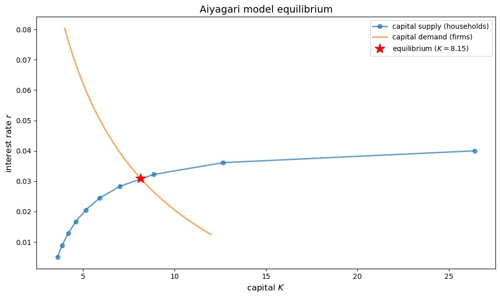
Equilibrium capital: 8.1484
Equilibrium interest rate: 0.0309
Equilibrium wage: 1.3388
90.5.1. Visualizing equilibrium#
Let’s plot the supply and demand curves:
# Supply curve: capital supplied by households as a function of r
r_vals = np.linspace(0.005, 0.04, 10)
K_supply_vals = []

for r in r_vals:
    w = r_to_w(r, firm)
    prices = Prices(r=r, w=w)
    K_supply_vals.append(capital_supply(household, prices, key))

# Demand curve: capital demanded by firms as a function of r
K_vals = np.linspace(4, 12, 50)
r_demand_vals = r_given_k(K_vals, firm)

fig, ax = plt.subplots(figsize=(10, 6))

ax.plot(K_supply_vals, r_vals, 'o-', lw=2, alpha=0.7,
        label='capital supply (households)', markersize=6)
ax.plot(K_vals, r_demand_vals, lw=2, alpha=0.7,
        label='capital demand (firms)')
ax.plot(K_star, r_star, 'r*', markersize=15, zorder=5,
        label=f'equilibrium ($K={K_star:.2f}$)')

ax.set_xlabel('capital $K$', fontsize=12)
ax.set_ylabel('interest rate $r$', fontsize=12)
ax.set_title('Aiyagari model equilibrium', fontsize=14)
ax.legend(fontsize=10)

plt.tight_layout()
plt.show()
90.6. Wealth Distribution#
One advantage of the simulation approach is that we can easily examine the wealth distribution.
We reuse the cross-section simulated at equilibrium prices:
prices_star = Prices(r=r_star, w=w_star)
σ_star = solve_household(household, prices_star)
assets_dist, z_dist = simulate_cross_section(σ_star, household, prices_star, key)

assets_dist = np.asarray(assets_dist)
We use QuantEcon’s lorenz_curve and gini_coefficient to summarize inequality:
fig, axes = plt.subplots(1, 2, figsize=(14, 5))

# Histogram
ax = axes[0]
ax.hist(assets_dist, bins=50, density=True, alpha=0.7, edgecolor='black')
ax.axvline(np.mean(assets_dist), color='red', linestyle='--', linewidth=2,
           label=f'mean = {np.mean(assets_dist):.3f}')
ax.axvline(np.median(assets_dist), color='orange', linestyle='--', linewidth=2,
           label=f'median = {np.median(assets_dist):.3f}')
ax.set_xlabel('assets', fontsize=12)
ax.set_ylabel('density', fontsize=12)
ax.set_title('Wealth distribution', fontsize=14)
ax.legend()

# Lorenz curve
ax = axes[1]
cum_pop, cum_wealth = qe.lorenz_curve(assets_dist)
ax.plot(cum_pop, cum_wealth, lw=2, label='Lorenz curve')
ax.plot([0, 1], [0, 1], 'k--', lw=1, alpha=0.5, label='perfect equality')
ax.set_xlabel('cumulative population share', fontsize=12)
ax.set_ylabel('cumulative wealth share', fontsize=12)
ax.set_title('Lorenz curve', fontsize=14)
ax.legend()

plt.tight_layout()
plt.show()

gini = qe.gini_coefficient(assets_dist)
print(f"\nGini coefficient: {gini:.4f}")
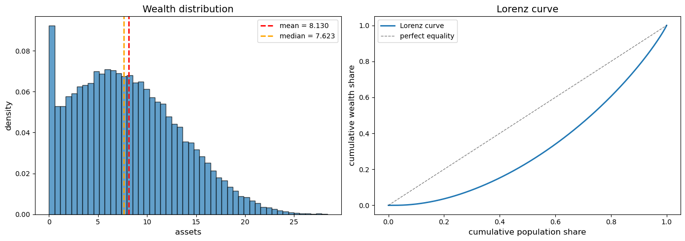
Gini coefficient: 0.3645
90.7. Summary and Comparison#
This lecture demonstrated how to solve the Aiyagari model using:
Endogenous Grid Method (EGM) for the household problem
avoids costly root-finding by working backwards from the Euler equation
directly computes consumption from marginal utility
more efficient than value function iteration
Simulation for computing aggregate capital
simulates a large cross-section of households
more flexible than analytical stationary distributions
allows easy computation of wealth inequality measures
90.7.1. Comparison with standard approach#
Compared to the standard Aiyagari lecture:
Advantages:
EGM avoids the root-finding required by value function iteration
simulation is more flexible (works with continuous shocks, non-linear policies)
it is easy to compute distributional statistics (Gini, percentiles, etc.)
the approach is simpler to extend to more complex models
Disadvantages:
simulation requires a large number of households for accuracy
equilibrium computation is subject to Monte Carlo noise
it is less precise than the analytical stationary distribution
90.7.2. Extensions#
This framework can be easily extended to:
continuous income shocks (e.g., lognormal)
more complex preference specifications
aggregate shocks and heterogeneous agent New Keynesian (HANK) models
life-cycle models with age-dependent policies
90.8. Exercises#
Exercise 90.1
Compare the speed and accuracy of EGM against the value function iteration approach used in the standard Aiyagari lecture.
Solve the household problem with both methods at the same prices.
Time both methods and compare the resulting policies.
Which method is faster? Are the policies close?
Exercise 90.2
Study how the wealth distribution changes with the discount factor \(\beta\).
Compute equilibria for \(\beta \in \{0.94, 0.95, 0.96, 0.97\}\).
For each \(\beta\), compute and plot the wealth distribution.
How does the Gini coefficient change with \(\beta\)?
Explain the economic intuition.
Exercise 90.3
The simulation method introduced in this lecture uses a fixed number of periods. Investigate the impact of this choice:
Vary
num_periodsfrom 200 to 2000.For each value, compute the mean assets multiple times with different random keys.
Plot the standard deviation of the capital estimate as a function of
num_periods.What is the trade-off between accuracy and computational cost?
Exercise 90.4
Extend the model to include a third employment state (e.g., unemployed, part-time, full-time):
Set up a 3-state Markov chain with appropriate transition probabilities.
Define income levels for each state.
Re-compute the equilibrium.
How does the additional heterogeneity affect the wealth distribution?